In our earliest work on dynamic algorithm configuration (DAC) we introduced the framework itself and presented the formulation of dynamic configuration as a contextual Markov Decision Process (cMDP). Based on this formulation, we proposed and evaluated solution approaches based on reinforcement learning.
To properly study the effectiveness and limitations of these approaches, we introduced artificial benchmarks that have very low computational overhead while enabling evaluation of DAC policies with full control over all aspects and characteristics of the environment. Specifically, we designed the Sigmoid and Luby benchmarks.
Sigmoid, as the name implies, is based on the sigmoid function $latex sig(t) = \frac{1}{1 + e^{-t}}$.
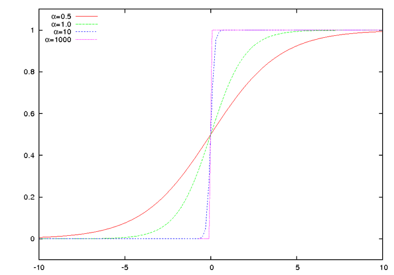
Effect of the scaling factor (here $latex \alpha$) on sigmoid functions all with inflection point $latex 0$. (Original from Wikimedia)
However, to allow for the notion of problem instances in this benchmark, we introduced the notion of context features.
These features (aka meta-features in other settings) enable us to easily distinguish one problem instance from another.
For example, the feature “height” would let help you distinguish mountains from each other.
For Sigmoid the context features are the scaling factor $latex s_{i, h}$ and the inflection point $latex p_{i, h}$, which depend on the problem instance at hand $latex i$ and the hyperparameter dimension $latex h$. With these features, we can construct complex Sigmoid functions that are shifted along the time axis $latex t$ and exhibit different scaling factors. Further, by basing the context features on the hyperparameter dimension, we can study the ability of dynamic configuration policies in configuring multiple parameters at once.
The resulting Sigmoid thus is $latex sig(t; s_{i, h},p_{i, h})= \frac{1}{1 + e^{-s_{i, h}\cdot(t – p_{i, h})}}$.
The second benchmark Luby is based on the luby sequence which is 1,1,2,1,1,2,4,1,1,2,1,1,2,4,8,…; formally, thet-th value inthe sequence can be computed as:
$latex l_t = \left\{\begin{array}{ll}2^{k-1}& \mathrm{if }\,t = 2^k – 1,\\l_{t – 2^{k – 1} + 1}& \mathrm{if }\,2^{k-1}\leq t < 2^k – 1.\end{array}\right.$
Again we can introduce context features to modify the original sequence. For example, we introduced a “short effective sequence length” $latex L$. This value tells us how many correct actions need to be played before an instance is deemed solved. Every incorrect choice will than require at least one additional action to counteract the wrong choices.
If you want to play around with the proposed benchmarks and some simple RL agents that can learn to solve them,
checkout the source code. You can also checkout the video presentation at ECAI’20:
References
- A. Biedenkapp and H. F. Bozkurt and T. Eimer and F. Hutter and M. Lindauer
Dynamic Algorithm Configuration: Foundation of a New Meta-Algorithmic Framework
In: Proceedings of ECAI20
Link to source code of usage of DAC on artificial benchmarks. Link to accompanying blog post.
Link to the video presentation at ECAI’20. - A. Biedenkapp and H. F. Bozkurt and F. Hutter and M. Lindauer
Towards White-box Benchmarks for Algorithm Control
In: DSO Workshop@IJCAI’19
Note: In this early work we referred to DAC as “Algorithm Control”